| Method | What it answers |
|---|---|
| PCA | Where does most of the variance in my spectra come from? Are there outliers? |
| t-SNE | Are there natural clusters in my data when I look at it in 2D? |
| K-Means | If I assume there are N groups, what does that grouping look like? |
Analysis vs run
The unsupervised feature has two levels:| Concept | Description |
|---|---|
| Analysis | A workspace tied to one sensor. Holds a set of related runs you want to compare. |
| Run | A single execution of one method (PCA, t-SNE, or K-Means) with a specific preprocessing pipeline and parameters. |
Creating an analysis
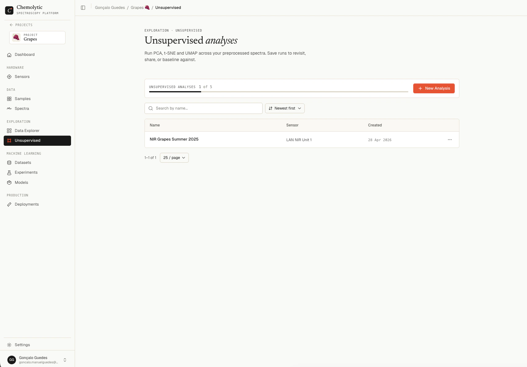
Click New analysis on the Unsupervised page.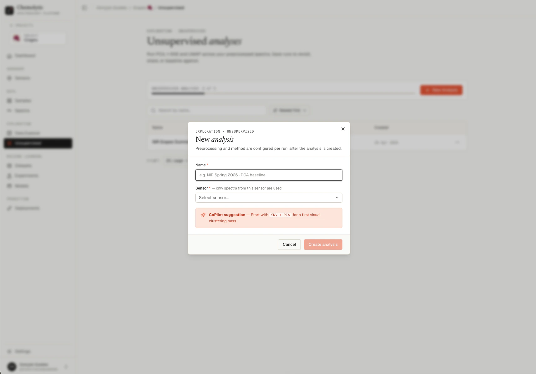
| Field | Required | Notes |
|---|---|---|
| Name | Yes | A descriptive label (e.g., “NIR Spring 2026 · PCA baseline”) |
| Sensor | Yes | Only spectra from this sensor are included |
Analysis detail page
The detail page has three main sections:- Spectra preview: apply preprocessing and visualize the resulting spectra before committing to a run
- Configure run: pick a method and parameters, then launch
- Runs list: see all runs in this analysis, their status, and open them
Spectra preview
Before committing to a run, you can interactively apply preprocessing and watch the spectra change. This is the fastest way to find a pipeline that brings out the structure in your data. The Spectra preview card has two parts:- Spectral overlay chart on the left: every active spectrum overlaid
- Preprocessing pipeline sidebar on the right: the catalog of methods you can apply
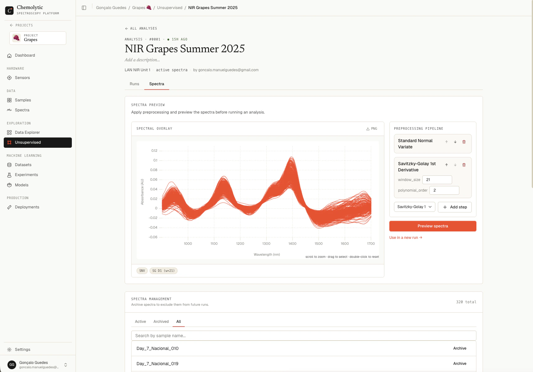
Building a pipeline
The pipeline is a list of preprocessing steps, applied in order. Each step’s output feeds the next step’s input.Pick a method from the catalog
The catalog groups methods by category (Smooth, Baseline, Scatter, Derivative, Scale). Click a method to add it to the pipeline.
Reorder steps if needed
Drag a step up or down to change the order. Order matters: SNV → SG D1 produces a different result than SG D1 → SNV.
Preview the result
Click Preview spectra. The chart updates to show your spectra after the pipeline is applied. The original raw spectra are not modified.
Reading the chart
The preview chart shows all active (non-archived) spectra overlaid. Hover any line to highlight it. The x-axis uses the sensor’s units (e.g., nm or cm⁻¹), the y-axis depends on the last step in the pipeline (e.g., absorbance for raw or SNV, derivative units for SG D1). What to look for as you tweak the pipeline:| Observation | What it suggests |
|---|---|
| Lines collapse to one shape, individual differences gone | You’ve over-smoothed or over-corrected. Remove a step. |
| Lines spread out into clear groups when coloured by sample | The pipeline is amplifying useful structure. Good sign. |
| Baseline drift removed (flat low region) | Your baseline correction is working |
| Sharp peaks become more visible | A derivative is helping |
| Noise removed (smoother lines) | Smoothing is working |
Available methods
| Category | Methods | Purpose |
|---|---|---|
| Smooth | SG Smooth, Mean filter, Median filter, Whittaker | Remove high-frequency noise |
| Baseline | Linear baseline, AirPLS, ArPLS | Remove baseline drift |
| Scatter | SNV, MSC, RNV | Correct for light scattering and path length |
| Derivative | SG D1, SG D2, Norris D1, Norris D2 | Enhance peaks, remove baselines |
| Scale | Mean center, Autoscale, Pareto, MinMax, Norm | Standardize variables before modelling |
Categories are mostly exclusive: you typically use one method per category. The UI prevents you from adding two baseline methods to the same pipeline, for example.
Common pipelines
| Pipeline | When to use |
|---|---|
| SNV → Mean center | A safe default for most NIR/FTIR data |
| SG D1 → Mean center | When you have baseline drift but not much scatter |
| MSC → SG D2 → Autoscale | When scatter and overlapping peaks are both problems |
From preview to a run
When the preview looks good, click Use in a new run → at the bottom of the preview card. This carries the pipeline directly into the Configure run form below, so you don’t have to rebuild it. Pick a method, set parameters, and launch.Spectra management
You can archive specific spectra to exclude them from future runs (useful for outliers identified by PCA). The archive list on the detail page mirrors the global Spectra page but scoped to this analysis. Archived spectra do not participate in new runs but the existing runs that already used them remain unchanged.Plan limits
Your plan limits the total number of analyses you can have. The current count and limit appear on the Analyses page. If you’ve reached the limit, delete an analysis you no longer need before creating a new one.What’s next
Now that you’ve configured a preprocessing pipeline, choose a method:- PCA for variance and outlier detection
- t-SNE for 2D cluster visualization
- K-Means to group samples into N clusters
- Comparing runs when you have multiple runs to compare