Before diving into the guides, it helps to understand how Chemolytic organizes your work. Here’s the big picture:
Organizations and projects
Organizations are your top-level workspace. Think of them as your company or team. Every user gets a personal organization when they sign up.
Projects live inside organizations. Each project is an independent workspace for a specific use case: “Olive Oil Quality”, “Cement Analysis”, “Polymer Identification”.
Sensors
A sensor represents the physical spectrometer you used to measure your samples. Chemolytic needs to know about your sensor because:
- Different sensors produce spectra with different wavelength ranges and number of data points
- Spectra from different sensors are not directly comparable
- When deploying a model, it must know which sensor produced the input spectra
Chemolytic supports these spectroscopy types:
| Type | Full name | Typical use |
|---|
| NIR | Near-Infrared | Food quality, pharmaceuticals, agriculture |
| FTIR | Fourier-Transform Infrared | Chemical identification, polymers, organic compounds |
| SWIR | Short-Wave Infrared | Remote sensing, minerals, moisture |
| Raman | Raman Spectroscopy | Materials science, forensics, pharmaceuticals |
| UV-Vis | Ultraviolet-Visible | Concentration analysis, color measurement |
You don’t need to understand the physics of spectroscopy to use Chemolytic. Just pick the type that matches your instrument.
Samples
A sample is a physical item you measured: an olive oil bottle, a soil core, a tablet, a grain batch. Each sample has:
- A name (e.g., “Sample-001”)
- An optional description
- One or more property values (the things you want to predict)
Properties
Properties are the characteristics of your samples that you want to predict from spectra. There are two types:
Continuous properties
Numeric values on a scale. Examples:
- Moisture content (%)
- Protein concentration (mg/mL)
- Acidity (pH)
- Fat content (% w/w)
Continuous properties lead to regression models (predicting a number).
Categorical properties
Discrete categories or labels. Examples:
- Quality grade (A, B, C)
- Origin (Brazil, Colombia, Ethiopia)
- Pass/Fail
- Material type (Plastic, Metal, Wood)
Categorical properties lead to classification models (predicting a category).
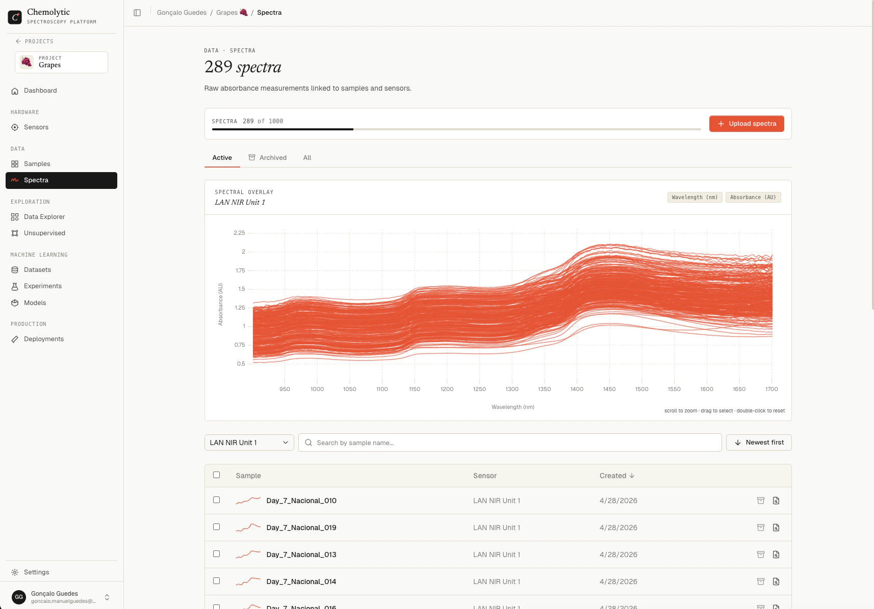
Spectra
A spectrum is the measurement output from your sensor for a given sample. It’s a series of intensity values across wavelengths or wavenumbers, essentially a curve.
In Chemolytic, spectra are:
- Uploaded as CSV files
- Always linked to a sensor (so Chemolytic knows the x-axis scale)
- Linked to a sample (so Chemolytic knows which physical item was measured)
- Visualized as interactive line charts
Each spectrum must come from one sensor. You cannot mix spectra from different instruments in the same upload batch.
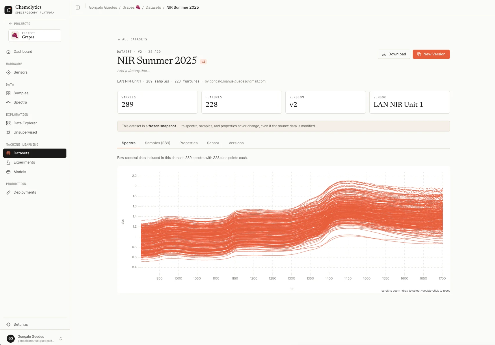
Datasets
A dataset is a packaged collection of spectra and sample properties, ready for modelling. Think of it as the “input” to an experiment.
When you create a dataset, Chemolytic:
- Takes spectra from a specific sensor
- Matches them with their sample properties
- Creates a manifest (a table showing which spectrum pairs with which sample and property values)
- Freezes this snapshot so your experiment results are reproducible
Datasets can be versioned. If you add new samples or fix property values, you can create a new version without losing the original.
Preprocessing
Raw spectra often contain noise, baseline drift, or scaling differences. Preprocessing cleans and transforms spectra before modelling.
| Method | What it does | When to use |
|---|
| SNV | Normalizes each spectrum to zero mean, unit variance | Corrects for light scattering, path length differences |
| MSC | Corrects scatter by fitting to a reference spectrum | Similar to SNV, for diffuse reflectance |
| SG D1 | Smooths and takes the first derivative | Removes baseline offset, enhances peaks |
| SG D2 | Smooths and takes the second derivative | Resolves overlapping peaks, removes linear baseline |
| Mean center | Subtracts the mean spectrum from all spectra | Standard step for most models |
| Autoscale | Mean centers then scales each variable to unit variance | When variables have very different magnitudes |
Don’t know which preprocessing to use? Use CoPilot mode and it will test all relevant combinations automatically.
Experiments
An experiment is where you build predictive models. You give it a dataset and a target property, and it produces trials. Each trial is one model trained with a specific preprocessing pipeline and algorithm.
Two modes
| Mode | Best for | What happens |
|---|
| CoPilot | Beginners, quick results | Automatically tests 250+ combinations of preprocessing and models, picks the best |
| Scientist | Experts, specific configurations | You manually choose preprocessing steps and algorithm for full control |
Available model algorithms
| Algorithm | Abbreviation | Type |
|---|
| Partial Least Squares | PLS | Regression & Classification |
| Principal Component Regression | PCR | Regression |
| Ridge Regression | Ridge | Regression & Classification |
| K-Nearest Neighbors | KNN | Regression & Classification |
| Support Vector Machine | SVR | Regression & Classification |
| Random Forest | RF | Regression & Classification |
Models
When an experiment finishes, you can register the best trial as a named model in the Model Registry. Registered models:
- Have a name and version number
- Track their performance metrics (R², RMSE, accuracy, etc.)
- Pin to the dataset version they were trained on for reproducibility
- Can be deployed as prediction endpoints
- Support versioning: train a new version without losing the old one
Deployments
A deployment puts a registered model into production. Once deployed, you can:
- Send new spectra and get predictions back instantly via the web interface
- Generate API keys for programmatic predictions
- Track which sensors the deployment supports
- Activate/deactivate without deleting the deployment or its logs
The full workflow
Set up your sensor
Tell Chemolytic what instrument you’re using.
Create samples and properties
Define what you measured and what you want to predict.
Upload spectra
Import your spectral data files and link them to samples.
Explore (optional)
Run PCA or clustering to understand your data before modelling.
Create a dataset
Bundle spectra and properties into a modelling-ready package.
Run an experiment
Let CoPilot find the best model, or configure it yourself in Scientist Mode.
Register the best model
Save it to the Model Registry for tracking and deployment.
Deploy and predict
Put the model live and start getting predictions on new data.