> ## Documentation Index
> Fetch the complete documentation index at: https://docs.chemolytic.com/llms.txt
> Use this file to discover all available pages before exploring further.
# Scientist mode
> Hand-configured experiments. Submit jobs one at a time with full control over preprocessing, models, and hyperparameter search.
Scientist mode is the manual counterpart to CoPilot. Instead of one big automated search, you submit **jobs** one at a time and decide exactly what each one tries.
## When to use Scientist mode
Pick Scientist mode when:
* You know the preprocessing or model you want and just need to run it
* You're benchmarking a specific configuration against other approaches
* CoPilot didn't converge or you want to override its choices
* You're testing a paper's recipe or reproducing literature results
* You want to try a model family CoPilot excluded (e.g., RF on a small dataset)
## The Scientist workflow
A Scientist experiment stays in **Active** status forever. You add jobs, watch them complete, look at the results, and decide what to try next.
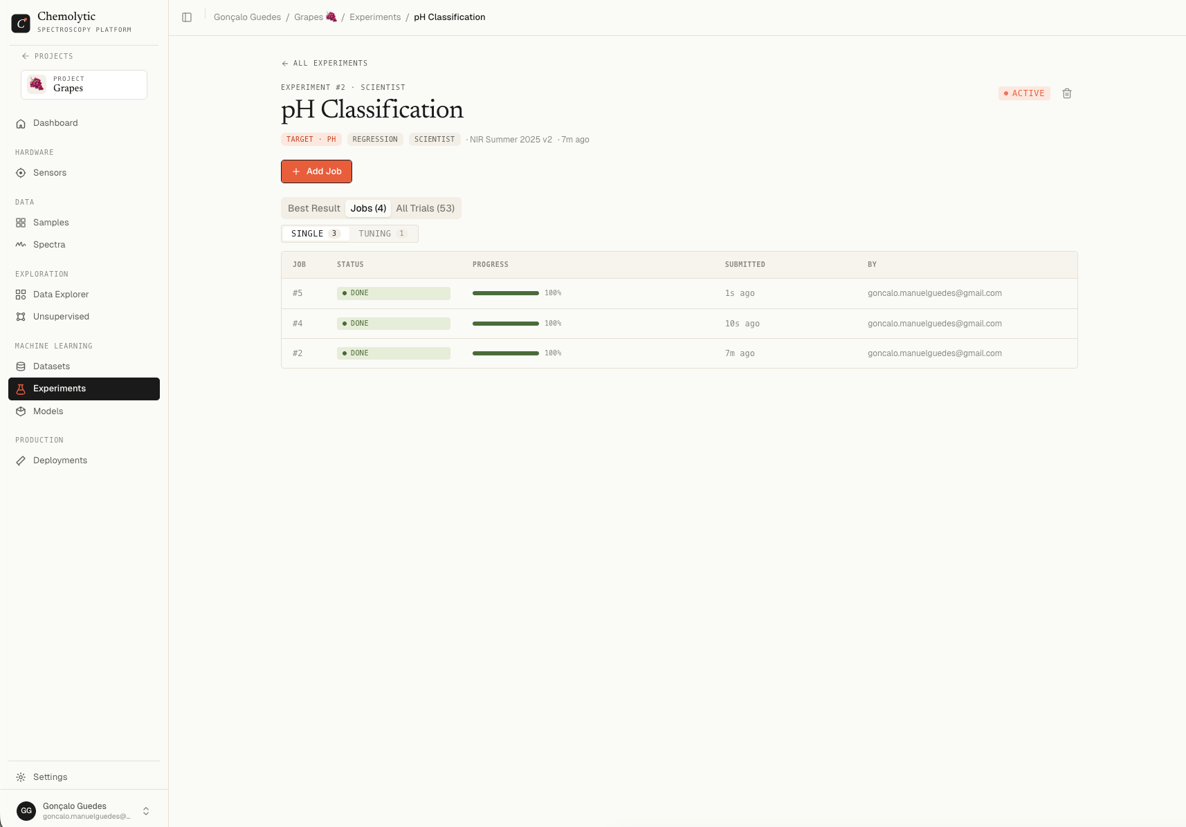 The detail page has up to three tabs:
| Tab | When it appears |
| --------------- | ------------------------ |
| **Best result** | Once any trial succeeds |
| **Jobs** | Always |
| **All trials** | Once any trial completes |
## Adding a job
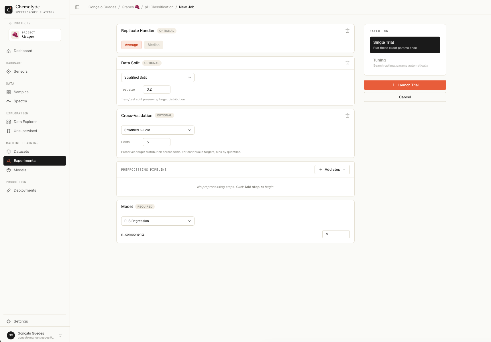
Click **+ Add Job** in the top right of the detail page.
The detail page has up to three tabs:
| Tab | When it appears |
| --------------- | ------------------------ |
| **Best result** | Once any trial succeeds |
| **Jobs** | Always |
| **All trials** | Once any trial completes |
## Adding a job
Click **+ Add Job** in the top right of the detail page.
 ### Job type
Two options:
| Type | What it does | Trial count |
| ---------- | ---------------------------------------------------- | --------------------- |
| **Single** | Runs one trial with the exact params you specify | 1 |
| **Tuning** | Searches a parameter space, runs N trials via Optuna | 2 to 500 (default 50) |
Each completed job (whether 1 trial or 50) counts as **one** against your monthly Scientist quota.
### Preprocessing pipeline
Click **+ Add step** to open the catalog. Steps are grouped by category:
| Category | Methods |
| ---------------------- | ---------------------------------------------- |
| **Scatter Correction** | SNV, MSC |
| **Derivatives** | SG D1, SG D2 |
| **Baseline** | (Linear baseline, AirPLS, ArPLS in some plans) |
| **Scaling** | Mean Center, Autoscale |
Each step you add appears in order. You can reorder by dragging. Some steps have parameters:
| Step | Parameters |
| --------------------------- | -------------------------------------------------------- |
| **SG D1** | window\_size (default 21), polynomial\_order (default 2) |
| **SG D2** | window\_size, polynomial\_order |
| **SNV / MSC** | None |
| **Mean Center / Autoscale** | None |
Order matters. SNV → SG D1 produces a different model than SG D1 → SNV. The conventional order is **scatter → derivative → scaling**.
### Model selection
Pick one algorithm. Options depend on the experiment type.
#### Regression models
| Model | Hyperparameters |
| ---------------------------------------- | --------------------------------------------- |
| **PLS** (Partial Least Squares) | n\_components (1-20) |
| **PCR** (Principal Component Regression) | n\_components (1-20) |
| **Ridge** | alpha (0.001 - 1000) |
| **KNN** | n\_neighbors (1-20) |
| **SVR** | C, epsilon, kernel |
| **RF** (Random Forest) | n\_estimators, max\_depth, min\_samples\_leaf |
#### Classification models
| Model | Hyperparameters |
| ----------------------- | --------------------------------------------- |
| **PLS-DA** | n\_components (1-20) |
| **Logistic Regression** | C (regularization strength) |
| **KNN** | n\_neighbors (1-20) |
| **SVM** | C, kernel |
| **RF** | n\_estimators, max\_depth, min\_samples\_leaf |
### Single trial: exact params
For a Single job, fill in each hyperparameter with one value. The trial uses exactly those numbers.
Example: PLS with n\_components = 8.
### Tuning job: parameter ranges
For a Tuning job, you define a **search space** for each hyperparameter. Two modes per param:
| Mode | When to use |
| ----------- | -------------------------------------------------- |
| **Fixed** | Lock the param to one value |
| **Range** | Tune within (min, max) for numeric params |
| **Choices** | Tune across a set of values for categorical params |
Set the **N trials** field (default 50). Optuna explores the search space, focusing on regions that produce good metrics.
Example: Tuning PLS with n\_components Range (1-20), n\_trials = 50. Optuna runs 50 trials with different n\_components values, learning which range gives the best CV metric.
## Following progress
A running job appears at the top of the detail page in a flame-coloured banner showing:
* Job ID
* Job type (single or tuning)
* Trials completed / total
* Progress percentage
The banner updates live every 3 seconds.
## Jobs tab
Two sub-tabs: **Single** and **Tuning**.
| Column | Description |
| ------------- | ---------------------------------- |
| **Job ID** | Sequential number |
| **Status** | Pending, Running, Done, Failed |
| **Trials** | "X/Y" for tuning, "1/1" for single |
| **Progress** | Bar with percentage |
| **Submitted** | Relative time |
| **By** | User email |
Click any successful tuning job to expand its trial leaderboard inline.
## All trials tab
Aggregated leaderboard across all jobs in this experiment. Shows the same columns as the per-job leaderboard.
This is useful for:
* Comparing trials across different jobs
* Sorting by any metric
* Filtering by model family
### Table view vs Parallel view
A toggle at the top switches between two visualizations:
| View | Best for |
| ------------------------ | ----------------------------------------------------------------------------------- |
| **Table** | Direct comparison of metrics, sorting, finding outliers |
| **Parallel coordinates** | Spotting which preprocessing + model + hyperparameter combinations cluster together |
In parallel coordinates, each line is a trial. Each axis is a parameter or metric. You can hover to highlight a trial or click to open its detail.
## Iteration tips
**Start with a single trial of CoPilot's recommendation.** Use the same preprocessing and model that CoPilot picked. Confirm you can reproduce the result manually. From there, vary one thing at a time.
**Use tuning jobs to explore.** A tuning job with 30-50 trials over a wide hyperparameter range is the fastest way to find a good local optimum. Then run a single trial with the best params to lock it in.
**Don't run too many trials in one job.** Tuning jobs over 100 trials are slow and rarely improve much beyond 30-50. Start small and add more only if needed.
## Job vs trial quotas
Each **job** counts as one against your monthly Scientist quota. The number of trials inside a job doesn't affect the quota.
This means a tuning job with 100 trials uses the same quota as a single trial.
## Best result tab
Once any trial succeeds, the **Best result** tab appears. It shows the same metric grid and chart as in CoPilot: predicted vs actual (regression) or confusion matrix (classification).
The "best" trial is selected automatically based on the primary metric (RMSE for regression, F1 macro for classification). You can register any trial as a model, not just the best one.
## Registering a model
When a trial looks good:
1. Click the trial in the leaderboard
2. The trial detail modal opens
3. Click **Register Model**
See [Trial results](/modelling/trial-results) for the registration flow in detail.
### Job type
Two options:
| Type | What it does | Trial count |
| ---------- | ---------------------------------------------------- | --------------------- |
| **Single** | Runs one trial with the exact params you specify | 1 |
| **Tuning** | Searches a parameter space, runs N trials via Optuna | 2 to 500 (default 50) |
Each completed job (whether 1 trial or 50) counts as **one** against your monthly Scientist quota.
### Preprocessing pipeline
Click **+ Add step** to open the catalog. Steps are grouped by category:
| Category | Methods |
| ---------------------- | ---------------------------------------------- |
| **Scatter Correction** | SNV, MSC |
| **Derivatives** | SG D1, SG D2 |
| **Baseline** | (Linear baseline, AirPLS, ArPLS in some plans) |
| **Scaling** | Mean Center, Autoscale |
Each step you add appears in order. You can reorder by dragging. Some steps have parameters:
| Step | Parameters |
| --------------------------- | -------------------------------------------------------- |
| **SG D1** | window\_size (default 21), polynomial\_order (default 2) |
| **SG D2** | window\_size, polynomial\_order |
| **SNV / MSC** | None |
| **Mean Center / Autoscale** | None |
Order matters. SNV → SG D1 produces a different model than SG D1 → SNV. The conventional order is **scatter → derivative → scaling**.
### Model selection
Pick one algorithm. Options depend on the experiment type.
#### Regression models
| Model | Hyperparameters |
| ---------------------------------------- | --------------------------------------------- |
| **PLS** (Partial Least Squares) | n\_components (1-20) |
| **PCR** (Principal Component Regression) | n\_components (1-20) |
| **Ridge** | alpha (0.001 - 1000) |
| **KNN** | n\_neighbors (1-20) |
| **SVR** | C, epsilon, kernel |
| **RF** (Random Forest) | n\_estimators, max\_depth, min\_samples\_leaf |
#### Classification models
| Model | Hyperparameters |
| ----------------------- | --------------------------------------------- |
| **PLS-DA** | n\_components (1-20) |
| **Logistic Regression** | C (regularization strength) |
| **KNN** | n\_neighbors (1-20) |
| **SVM** | C, kernel |
| **RF** | n\_estimators, max\_depth, min\_samples\_leaf |
### Single trial: exact params
For a Single job, fill in each hyperparameter with one value. The trial uses exactly those numbers.
Example: PLS with n\_components = 8.
### Tuning job: parameter ranges
For a Tuning job, you define a **search space** for each hyperparameter. Two modes per param:
| Mode | When to use |
| ----------- | -------------------------------------------------- |
| **Fixed** | Lock the param to one value |
| **Range** | Tune within (min, max) for numeric params |
| **Choices** | Tune across a set of values for categorical params |
Set the **N trials** field (default 50). Optuna explores the search space, focusing on regions that produce good metrics.
Example: Tuning PLS with n\_components Range (1-20), n\_trials = 50. Optuna runs 50 trials with different n\_components values, learning which range gives the best CV metric.
## Following progress
A running job appears at the top of the detail page in a flame-coloured banner showing:
* Job ID
* Job type (single or tuning)
* Trials completed / total
* Progress percentage
The banner updates live every 3 seconds.
## Jobs tab
Two sub-tabs: **Single** and **Tuning**.
| Column | Description |
| ------------- | ---------------------------------- |
| **Job ID** | Sequential number |
| **Status** | Pending, Running, Done, Failed |
| **Trials** | "X/Y" for tuning, "1/1" for single |
| **Progress** | Bar with percentage |
| **Submitted** | Relative time |
| **By** | User email |
Click any successful tuning job to expand its trial leaderboard inline.
## All trials tab
Aggregated leaderboard across all jobs in this experiment. Shows the same columns as the per-job leaderboard.
This is useful for:
* Comparing trials across different jobs
* Sorting by any metric
* Filtering by model family
### Table view vs Parallel view
A toggle at the top switches between two visualizations:
| View | Best for |
| ------------------------ | ----------------------------------------------------------------------------------- |
| **Table** | Direct comparison of metrics, sorting, finding outliers |
| **Parallel coordinates** | Spotting which preprocessing + model + hyperparameter combinations cluster together |
In parallel coordinates, each line is a trial. Each axis is a parameter or metric. You can hover to highlight a trial or click to open its detail.
## Iteration tips
**Start with a single trial of CoPilot's recommendation.** Use the same preprocessing and model that CoPilot picked. Confirm you can reproduce the result manually. From there, vary one thing at a time.
**Use tuning jobs to explore.** A tuning job with 30-50 trials over a wide hyperparameter range is the fastest way to find a good local optimum. Then run a single trial with the best params to lock it in.
**Don't run too many trials in one job.** Tuning jobs over 100 trials are slow and rarely improve much beyond 30-50. Start small and add more only if needed.
## Job vs trial quotas
Each **job** counts as one against your monthly Scientist quota. The number of trials inside a job doesn't affect the quota.
This means a tuning job with 100 trials uses the same quota as a single trial.
## Best result tab
Once any trial succeeds, the **Best result** tab appears. It shows the same metric grid and chart as in CoPilot: predicted vs actual (regression) or confusion matrix (classification).
The "best" trial is selected automatically based on the primary metric (RMSE for regression, F1 macro for classification). You can register any trial as a model, not just the best one.
## Registering a model
When a trial looks good:
1. Click the trial in the leaderboard
2. The trial detail modal opens
3. Click **Register Model**
See [Trial results](/modelling/trial-results) for the registration flow in detail.